Please tell me what you thought about this blog. Comments, suggestions and views are welcomed.

繼續閱讀全文　這是留言板-既然來了，就留個言再走吧！

• 編輯文章
• 此文章網址
• 轉寄此文章
• 目前有66 意見

A Sustainable Dynamic Optimization Model of Pricing and Advertising in the Presence of Green Innovation Investment

Chung-Yuan Dye and Tsu-Pang Hsieh

Finally, the acceptance from EJOR has arrived. The Julia code for the numerical examples in this paper is provided below. Alternatively, you can also implement it directly in Julia. Please leave a message if you have any problems with the implementation of the code.

julia=StartExternalSession["Julia"]

ExternalEvaluate[julia,"
using JuMP,Ipopt
dp(x)=(140-3*x);
K1(y)=(y/5-y^2/1000);
f1(x)=100*exp(-0.03*x);
f2(x)=2*exp(-0.045*x);
v1=25;
v2=10;
omega=300;
c=16.5;
h=0;
z=0.8;
"];

dynCP11=ExternalEvaluate[julia, "
	function dynCP11(G0,gamma1,gamma2,delta,k1coef,k2coef,e,r,varpi,n)
    m1 = Model(Ipopt.Optimizer) 
    set_silent(m1)
    #set_optimizer_attributes(m1, \"tol\" => 1e-4, \"max_iter\" => 100)
    register(m1, :dp, 1, dp; autodiff = true)
    register(m1, :K1, 1, K1; autodiff = true)
    register(m1, :f1, 1, f1; autodiff = true)
    register(m1, :f2, 1, f2; autodiff = true)
    @variable(m1, p[1:n], start = 30)
    @variable(m1, w[1:n], start = 10)
    @variable(m1, u[1:n], start = 10)

    @NLexpression(m1,newG[i=1:n],(1-delta)^(-1+i)*((1-delta)*G0
	+sum((gamma1*u[j+1]^k1coef+gamma2*w[j+1]^k2coef)/((1-delta)^j) 
    for j = 0:i-1)))
    
    @NLexpression(m1,newCE[i=1:n],f1(w[i])+f2(w[i])*dp(p[i])*K1(newG[i])-varpi)

    @NLobjective(
	m1,
	Max,
	sum(z^(i-1)*((p[i]-c-h/2)*dp(p[i])*K1(newG[i])
    -v1*u[i]^2/2-v2*w[i]^2/2-e*newCE[i])
                for i = 1:n))
	for i = 1:n
        @constraint(m1, p[i] >= c + h / 2)
	end
	for i = 1:n
        @constraint(m1, p[i] <= 140 / 3)
	end
	for i = 1:n
        @constraint(m1, w[i] >= 0)
	end
	for i = 1:n
        @constraint(m1, u[i] >= 0)
	end
	for i = 1:n
        @NLconstraint(m1, newCE[i] >= 0)
	end

	JuMP.optimize!(m1)

	p_val = JuMP.value.(p)
	w_val = JuMP.value.(w)
	u_val = JuMP.value.(u)

	G_val=(1-delta)*G0+gamma1*u_val[1]^k1coef+gamma2*w_val[1]^k2coef

	CE=f1(w_val[1])+f2(w_val[1])*dp(p_val[1])*K1(G_val)

	profit=(p_val[1]-c-h/2)*dp(p_val[1])*K1(G_val)
    -v1*u_val[1]^2/2-v2*w_val[1]^2/2-e*(CE-varpi)

	return[p_val,w_val,u_val,G_val,CE,profit,objective_value(m1)]

end"];

dynCP22=ExternalEvaluate[julia,"
	function dynCP22(G0,gamma1,gamma2,delta,k1coef,k2coef,e,r,varpi,n)
    m1 = Model(Ipopt.Optimizer) 
    set_silent(m1)
    #set_optimizer_attributes(m1, \"tol\" => 1e-4, \"max_iter\" => 100)
    register(m1, :dp, 1, dp; autodiff = true)
    register(m1, :K1, 1, K1; autodiff = true)
    register(m1, :f1, 1, f1; autodiff = true)
    register(m1, :f2, 1, f2; autodiff = true)
    @variable(m1, p[1:n], start = 30)
    @variable(m1, w[1:n], start = 10)
    @variable(m1, u[1:n], start = 10)

    @NLexpression(m1,newG[i=1:n],(1-delta)^(-1+i)*((1-delta)*G0
	+sum((gamma1*u[j+1]^k1coef+gamma2*w[j+1]^k2coef)/((1-delta)^j) 
    for j = 0:i-1)))
    
    @NLexpression(m1,newCE[i=1:n],f1(w[i])+f2(w[i])*dp(p[i])*K1(newG[i])-varpi)

    @NLobjective(
	m1,
	Max,
	sum(z^(i-1)*((p[i]-c-h/2)*dp(p[i])*K1(newG[i])
    -v1*u[i]^2/2-v2*w[i]^2/2-r*newCE[i])
                for i = 1:n))
	for i = 1:n
        @constraint(m1, p[i] >= c + h / 2)
	end
	for i = 1:n
        @constraint(m1, p[i] <= 140 / 3)
	end
	for i = 1:n
        @constraint(m1, w[i] >= 0)
	end
	for i = 1:n
        @constraint(m1, u[i] >= 0)
	end
	for i = 1:n
        @NLconstraint(m1, newCE[i] <= 0)
	end

	JuMP.optimize!(m1)

	p_val = JuMP.value.(p)
	w_val = JuMP.value.(w)
	u_val = JuMP.value.(u)

	G_val=(1-delta)*G0+gamma1*u_val[1]^k1coef+gamma2*w_val[1]^k2coef

	CE=f1(w_val[1])+f2(w_val[1])*dp(p_val[1])*K1(G_val)

	profit=(p_val[1]-c-h/2)*dp(p_val[1])*K1(G_val)
    -v1*u_val[1]^2/2-v2*w_val[1]^2/2-r*(CE-varpi)

	return[p_val,w_val,u_val,G_val,CE,profit,objective_value(m1)]

end"];

mysol13[g0_,\[Gamma]1_,\[Gamma]2_,\[Delta]_,k1_,k2_,e_,r_,cap_]:=
Block[{n=40,numiter=100,iter=0,ans1,ans2},
	Print[{Dynamic[iter],Dynamic[ans2]}];
	NestList[(
	iter=iter+1;
	ans1=
	SortBy[{
		dynCP11[#[[4]],\[Gamma]1,\[Gamma]2,\[Delta],k1,k2,e,r,cap,n],
		dynCP22[#[[4]],\[Gamma]1,\[Gamma]2,\[Delta],k1,k2,e,r,cap,n]},
          Last][[-1]];
	ans2={ans1[[1,1]],ans1[[2,1]],ans1[[3,1]],ans1[[4]],
          ans1[[5]],#[[-1]]+0.8^(iter-1)*ans1[[6]]})&,
	{0,0,0,g0,0,0},numiter][[2;;-1]]
]

myexample=mysol13[#[[1]],0.5,0.8,0.2,0.5,0.8,8,2,#[[2]]]&/@
Flatten[Table[{i,j},{j,{250,300,400}},{i,{10,40}}],1]

ListLinePlot[myexample[[All,All,#]],PlotRange->All,
Frame->True]&/@{1,2,3,4,5}//Column

繼續閱讀全文　Finally, the first acceptance of 2024 comes.

• 編輯文章
• 此文章網址
• 轉寄此文章
• 目前有0 意見

test=ImageData[Rasterize["50",RasterSize->50,ImageSize->200]]

data=ParallelTable[{i,j,If[Mean@test[[i,j]]>0.95,0,1]},
{i,Dimensions[test][[1]]},{j,Dimensions[test][[2]]}]

picdata=Table[ParallelMap[If[#[[-1]]==0,"",
ImageResize[Import[RandomChoice[FileNames["*.jpeg",
"/Users/chungyuandye/Pictures/照片圖庫V4.photoslibrary/originals/",Infinity]]],{100,100}]]&,
data[[i]]],{i,54}]

GraphicsGrid[picdata]

繼續閱讀全文　Mathematica 教學：Text arrangement

• 編輯文章
• 此文章網址
• 轉寄此文章
• 目前有0 意見

\documentclass{article}
\usepackage{tikz}
\usepackage{adjustbox}
\begin{document}
\begin{center}
\begin{adjustbox}{width=0.6\textwidth}
  \begin{tikzpicture}
  \pgfmathsetseed{42}
    \foreach \i in {1,...,500}
    {
      \pgfmathsetmacro{\a}{int(random(0,255))}
      \pgfmathsetmacro{\b}{int(random(0,255))}
      \pgfmathsetmacro{\c}{int(random(0,255))}
      \pgfmathsetmacro{\r}{rand*2}
      \pgfmathsetmacro{\x}{random(-10,10)}
      \pgfmathsetmacro{\y}{random(-10,10)}
      \definecolor{mycolor}{RGB}{\a,\b,\c}
      \fill[mycolor] (\x,\y) circle (\r cm);
    }
  \end{tikzpicture}
  \end{adjustbox}
  \end{center}
\end{document}

繼續閱讀全文　Tikz: Drawing Random Circles with Randomly Assigned Centers and Radii

• 編輯文章
• 此文章網址
• 轉寄此文章
• 目前有0 意見

session=StartExternalSession["Julia"]
test =
  "function testpi(size)
    sample = rand(size, 2)
    dist = broadcast(hypot, sample[:,1], sample[:,2])
    return sample, dist
end";
pitest=ExternalEvaluate[session,test]
size=100000
data=pitest[size];
ListPlot[GatherBy[Transpose[data[[1]]],Norm[#]<1&],Frame ->True,AspectRatio -> 1]
Length@GatherBy[Transpose[data[[1]]], Norm[#]<1&][[1]]/size//N




\documentclass[tikz]{standalone}
\usepackage{tikz}
\usepackage{ifthen}
\begin{document}
  \begin{tikzpicture}
	\draw[help lines, color=gray!30, dashed] (-1.2,1.5) grid (-1.2,1.5);
	\draw[->] (-1.2,0)--(1.1,0) node[right]{$x$};
	\draw[->] (0,-1.2)--(0,1.5) node[above]{$y$};
	\draw[domain=0:1, smooth, variable=\x, black] plot ({\x}, {sqrt(1-\x*\x)});
  \pgfmathsetseed{42}
    \foreach \i in {1,...,10000}
    {
      \pgfmathsetmacro{\x}{abs(rand)}
      \pgfmathsetmacro{\y}{abs(rand)}
      \pgfmathsetmacro{\r}{\x*\x+\y*\y}
       \pgfmathsetmacro{\col}{ifthenelse(\r<1,"blue!90","red!90")}
      \fill[\col] (\x,\y) circle (0.1pt)
      ;
    }
  \end{tikzpicture}
\end{document}

繼續閱讀全文　Mathematica 教學：Call Julia from Mathematica

• 編輯文章
• 此文章網址
• 轉寄此文章
• 目前有0 意見

 

Policy function iterations方法是通過計算出最佳化問題的每一步所實現的最佳結果，並將這些結果用於計算下一步的最佳結果。此過程在一定數量的迭代後會得到一個最佳策略，並且這個策略也是最終的最佳解。因此它對於解決複雜的最佳化問題非常有用。它可以被用於解決各種經濟學、工程學和其他領域的最佳化問題。

ClearAll["Global`*"]
\[Alpha]=0.3;
\[Beta]=0.95;
\[Delta]=0.1;
\[Sigma]=1.5;

size=99;

K=Range[0.1,5,4.9/(size)];
V=Table[0,{size}];


astHoward=With[{n=size},
obj=ParallelTable[If[i^\[Alpha]+(1-\[Delta])*i-j<0,-10^9,
((i^\[Alpha]+(1-\[Delta])*i-j)^(1-\[Sigma])-1)/(1-\[Sigma])],
{i,0.1,5,4.9/n},{j,0.1,5,4.9/n}];
loops=0;
\[Epsilon]=99999;

Print[Grid[{
{"loop number ",
Dynamic[loops],
" with distance ",
Dynamic[NumberForm[\[Epsilon],
ExponentFunction->(If[-10<#<10,Null,#]&)]]}}]];

NestWhile[
NestWhile[
Transpose@
Table[{obj[[i,#[[2,i]]]]+\[Beta]*#[[1,#[[2,i]]]],#[[2,i]]},{i,Length[#[[1]]]}]&,
Transpose[SortBy[#,First][[-1]]&/@
Table[{obj[[i,j]]+\[Beta]*#[[1,j]],j},{i,n+1},{j,n+1}]//Parallelize],
Norm[#1[[1]]-#2[[1]]]>10^-6&,2]&,
{Table[0,n+1],Table[0,n+1]},
(loops++;\[Epsilon]=Norm[#1[[1]]-#2[[1]]];
Norm[#1[[1]]-#2[[1]]]>10^-6)&,2]
]


astHowardMatrix=With[{n=size},
obj=ParallelTable[If[i^\[Alpha]+(1-\[Delta])*i-j<
0,-10^9,((i^\[Alpha]+(1-\[Delta])*i-j)^(1-\[Sigma])-1)/(1-\[Sigma])],
{i,0.1,5,4.9/n},{j,0.1,5,4.9/n}];
loops=0;
\[Epsilon]=99999;

Id=IdentityMatrix[size+1];

Print[Grid[{
{"loop number ",
Dynamic[loops],
" with distance ",
Dynamic[NumberForm[\[Epsilon],
ExponentFunction->(If[-10<#<10,Null,#]&)]]}}]];


NestWhile[
(
myValue=Transpose[SortBy[#,First][[-1]]&/@
Table[{obj[[i,j]]+\[Beta]*#[[1,j]],j},{i,n+1},{j,n+1}]//Parallelize];
{Inverse[(Id-\[Beta]*Normal[SparseArray[
Rule[#,1]&/@Transpose[
{Range[size+1],myValue[[2]]}],size+1]])].(obj[[#[[1]],#[[2]]]]&/@
Transpose[{Range[size+1],myValue[[2]]}]),myValue[[2]]}
)&,
{Table[0,n+1],Table[0,n+1]},
(loops++;\[Epsilon]=Norm[#1[[1]]-#2[[1]]];
Norm[#1[[1]]-#2[[1]]]>10^-6)&,2]
]


ListLinePlot[astHowardMatrix[[1]],PlotRange->All,AspectRatio->1,Frame->True]
ListLinePlot[astHowardMatrix[[2]],PlotRange->All,AspectRatio->1,Frame->True]

繼續閱讀全文　Mathematica 教學：Policy function iterations for deterministic cake eating problem

• 編輯文章
• 此文章網址
• 轉寄此文章
• 目前有0 意見

Value function iterations方法是通過計算出最佳化問題的每一步所實現的最佳結果，並將這些結果用於計算下一步的最佳結果。此過程在一定數量的迭代後會得到一個最佳策略，並且這個策略也是最終的最佳解。因此它對於解決複雜的最佳化問題非常有用。它可以被用於解決各種經濟學、工程學和其他領域的最佳化問題。

ClearAll["Global`*"]
\[Alpha]=0.3;
\[Beta]=0.95;
\[Delta]=0.1;
\[Sigma]=1.5;
size=99;
K=Range[0.1,5,4.9/(size)];
V=Table[0,{size}];

ast=With[{n=size},
obj=
ParallelTable[
If[i^\[Alpha]+(1-\[Delta])*i-j<0,-10^9,
((i^\[Alpha]+(1-\[Delta])*i-j)^(1-\[Sigma])-1)/(1-\[Sigma])],
{i,0.1,5,4.9/n},{j,0.1,5,4.9/n}];
loops=0;
\[Epsilon]=99999;

Print[
Grid[{{"loop number ",Dynamic[loops]," with distance ",
Dynamic[NumberForm[\[Epsilon],
ExponentFunction->(If[-10<#<10,Null,#]&)]]}}]];

NestWhile[
Transpose[SortBy[#,First][[-1]]&/@Table[{obj[[i,j]]+\[Beta]*#[[1,j]],
Range[0.1,5,4.9/n][[j]]},{i,n+1},{j,n+1}]//Parallelize]&,
{Table[0,n+1],Table[0,n+1]},(loops++;\[Epsilon]=Norm[#1[[1]]-#2[[1]]];
Norm[#1[[1]]-#2[[1]]]>10^-6)&,2]
];

繼續閱讀全文　Mathematica 教學：Value function iterations for deterministic cake eating problem

• 編輯文章
• 此文章網址
• 轉寄此文章
• 目前有0 意見

這是我這幾年來數量方法這一門課所自編的 Mathematica 入門教學講義。Mathematica 相較於其他軟體的特點在於強大的符號運算及動態幾何繪圖的科學運算能力。此外，Mathematica 尚包含數值運算、圖表可視化、動態操作介面等。由於擁有許多的內建程式語言及內建系統，故不需要繁雜且複雜的編寫，有能夠輕易上手的便利性。本教學講義相關檔案、資料檔及未來更新維護皆可由下列網址下載： 

https://github.com/chungyuandye/Mathematica

繼續閱讀全文　Mathematica 教學講義

• 編輯文章
• 此文章網址
• 轉寄此文章
• 目前有1 意見

 

帳號被盜走，上站6000次，我的青春啊！

2023年1月28日，失而復得。

繼續閱讀全文　青春啊！

• 編輯文章
• 此文章網址
• 轉寄此文章
• 目前有0 意見

JASP 統計軟體是由阿姆斯特丹大學 Eric-Jan Wagenmakers 教授領導的團隊，以 R 為核心所開發的 免費開源統計軟體，主要應用於心理及統計分析，相關的分析模組包含:平均數比較、實驗設計、迴歸與相關分析、探索性因素分析、驗證性因素分析（CFA）、結構方程式（SEM）、機械學習、神經網路等。

由於其設計理念為讓用戸熟悉並易於使用，故幾乎所有的分析模組都已視窗化，僅需要懂得相關的統計理論卽可輕易上手。有關 JASP 統計軟體的詳細説明可到官方網站參閲，https://jasp-stats.org/。JASP 統計軟體亦可由網站免費下載: 

https://jasp-stats.org/download/

本年度統計分析教材以JASP 講義為主，JASP 統計軟體除了是免費開源外，該軟體以視窗的為主，學生只要能了解課堂上講授的統計分析及進階的驗證性因素分析、競爭模式、多群組比較、結構方程模型的理論後，卽可輕易執行上手。此外，JASP 統計軟體所産生的報表 及圖形皆以 APA 格式輸出，學生也能因此免除在茫茫報表中重新整理資料、繪製圖形，簡化發 表硏究成果及撰寫論文的流程。本教材相關檔案、資料檔及未來更新維護皆可由下列網址下載:

https://github.com/chungyuandye/JASP-

繼續閱讀全文　用 JASP 輕鬆學 SEM:從基礎到應用

• 編輯文章
• 此文章網址
• 轉寄此文章
• 目前有0 意見

Mac PDF檔案縮小檔案大小：檔案➡輸出➡Quartz濾鏡➡Reduce file size。

繼續閱讀全文　Reduce PDF file size for Mac

• 編輯文章
• 此文章網址
• 轉寄此文章
• 目前有0 意見

利用三角板(30°-60°-90°)轉半圈即可。

pt[x0_]:={{0,0},{x0,Sqrt[4-x0^2]},{x,Sqrt[3-x^2]},{0,0}}/.
Quiet@Solve[{x^2+y^2==3,(x-x0)^2+(y-Sqrt[4-x0^2])^2==1},{x,y}][[2]]

Manipulate[
Plot[{Sqrt[4-x^2],Sqrt[3-x^2]},{x,-2,2},AspectRatio->1/2,
Epilog->{Green,Thickness[0.005],
Line[pt[Sqrt[3+10^(-7)]][[1;;3]]],
Red,PointSize[0.02],Point[pt[Sqrt[3+10^(-7)]]],
Point[pt[z][[1;;3]]],
Blue,Line[pt[z][[1;;2]]],Line[pt[z][[2;;3]]],
Line[pt[z][[3;;4]]]}
],{z,Sqrt[3]+10^(-7),-2}]

Integrate[Sqrt[4-x^2]-Sqrt[3-x^2],{x,0,Sqrt[3]}]

Integrate[Sqrt[4-x^2]-Sqrt[3](2+x),{x,-2,-(3/2)}]+
Integrate[Sqrt[4-x^2]-Sqrt[3-x^2],{x,-(3/2),Sqrt[3]}]//FullSimplify

繼續閱讀全文　111學測數A第18題

• 編輯文章
• 此文章網址
• 轉寄此文章
• 目前有1 意見

varimax[data_]:=Block[{AA,BB,CC,DD,nn,uu,XX,YY,vdata,angle,Tr,temp,vlist},
{nn,uu}=Dimensions[data];
vdata=Map[Normalize,data];
Do[
angle=Arg[nn* Total[Thread[Complex[
vdata[[All,iter[[1]]]],vdata[[All,iter[[2]]]]]]^4]
-Total[Thread[Complex[
vdata[[All,iter[[1]]]],vdata[[All,iter[[2]]]]]]^2]^2]/4;
Tr={{Cos[angle],-Sin[angle]},{Sin[angle],Cos[angle]}};
vdata[[All,iter]]= vdata[[All,iter]].Tr,
{iter,Flatten[Subsets[Range[uu],{2}]&/@Range[25],1]}
];
vdata*(Norm[#]&/@data)];


myfactor[data_]:=Block[{label,fadata,mypca,loadings,nf,rotatedloadings,
rotatedfactor,ncfa,proddata},
label=data[[1]];
fadata=data[[2;;-1]];
mypca=Eigensystem[Correlation@fadata];
nf=Length[Select[mypca[[1]],#>=1&]];
loadings=Transpose[mypca[[1,#]]^0.5*mypca[[2,#]]&/@Range[nf]];
rotatedloadings=varimax[loadings];
loadings=Flatten@{#,rotatedloadings[[#]],"",""}&/@Range[Length@loadings];
rotatedfactor=Table[Select[loadings,
(Abs[#[[i]]]==Max[Map[Abs,#[[2;;1+nf]]]])&],{i,2,nf+1}];
(rotatedfactor[[#,1,nf+2]]=mypca[[1,#]];
rotatedfactor[[#,1,nf+3]]=PercentForm[
Accumulate[mypca[[1]]][[#]]/Total[mypca[[1]]]];)&/@Range[nf];

Print["\n探索性因素分析\n"];

Print[TableForm[
Flatten[Table[Flatten@{StringReplace[label[[#[[1]]]]," "->""],
#[[2;;-1]]}&/@rotatedfactor[[i]],{i,nf}],1],
TableHeadings->{None, 
Flatten@{"題項","因素"<>ToString[#]&/@Range[nf],"特徵根","解釋百分比"}}]];
ncfa=Length/@rotatedfactor;
proddata=data[[All,Flatten[#[[All,1]]&/@rotatedfactor]]][[2;;-1]];

Print["\n驗證性因素分析\n"];

Print@thesisnoworrycfa[
proddata,ncfa,ToExpression["X"<>ToString[#]]&/@Range[nf]];
];

myfactorcheck[data_]:=Block[{label,fadata,mypca,loadings,nf,
rotatedloadings,rotatedfactor,ncfa,proddata,check,checkfactornum},
label=data[[1]];
fadata=data[[2;;-1]];
mypca=Eigensystem[Correlation@fadata];
nf=Length[Select[mypca[[1]],#>=1&]];
loadings=Transpose[mypca[[1,#]]^0.5*mypca[[2,#]]&/@Range[nf]];
rotatedloadings=varimax[loadings];
loadings=Flatten@{#,rotatedloadings[[#]],"",""}&/@Range[Length@loadings];
rotatedfactor=Table[Select[loadings,(Abs[#[[i]]]==Max[Map[Abs,#[[2;;1+nf]]]])&],{i,2,nf+1}];

rotatedfactor=Table[Insert[i,Length[rotatedfactor[[#]]],-1],
{i,rotatedfactor[[#]]}]&/@Range[Length[rotatedfactor]];

check[list_,j_]:=Block[{temp=list},
If[Abs[temp[[1+j]]]<0 .45="" actor="" nf="" temp="">ToString[j];
temp[[3+nf]]="因素負荷過低",temp[[2+nf]]="Factor "<>ToString[j];
temp[[3+nf]]=temp[[3+nf]]];temp];
 

check=Flatten[Select[#,#[[-2]]=="因素負荷過低"||#[[-1]]<=2&]&/@Table[
Map[check[#,i]&,rotatedfactor[[i]]],{i,nf}],1];
Print@TableForm@check;

data[[All,Complement[Range[Dimensions[data][[2]]],check[[All,1]]]]]
];

test=Import["test.xlsx"][[1]][[All,8;;29]];
semmethod="ML";
myfactor[NestWhile[myfactorcheck,test,UnsameQ,2]]

繼續閱讀全文　Mathematica 教學：Factor analysis with Varimax rotation

• 編輯文章
• 此文章網址
• 轉寄此文章
• 目前有0 意見

varimax[data_]:=
Block[{AA,BB,CC,DD,nn,uu,XX,YY,vdata,angle,Tr,temp,vlist},
{nn,uu}=Dimensions[data];
vdata=Map[Normalize,data];
Do[angle=Arg[nn*
Total[Thread[Complex[vdata[[All,iter[[1]]]],
vdata[[All,iter[[2]]]]]]^4]-
Total[Thread[Complex[vdata[[All,iter[[1]]]],
vdata[[All,iter[[2]]]]]]^2]^2]/4;
Tr={{Cos[angle],-Sin[angle]},{Sin[angle],Cos[angle]}};
vdata[[All,iter]]=vdata[[All,iter]].Tr,
{iter,Flatten[Subsets[Range[uu],{2}]&/@Range[25],1]}];
vdata*(Norm[#]&/@data)
]

L = {{-0.18444, 0.766739, -0.27758, 0.115158, 0.712221}, 
{0.698485, -0.30363, -0.19539, -0.2648, 0.688367}, 
{0.754094, 0.348652, -0.20205, -0.30588, 0.824599}, 
{0.365978, 0.162525, -0.1973, 0.849845, 0.92152}, 
{0.5781630, .044134, 0.452722, 0.157895, 0.566108},
{0.299667, 0.030388, 0.770856, 0.063739, 0.689006}, 
{0.817187, 0.239353, -0.19451, -0.16643, 0.79062}, 
{0.687893, 0.035304, 0.116032, 0.117627, 0.501742}, 
{0.301458, -0.74108, -0.3442, 0.233979, 0.81329}};
 

Map[NumberForm[#,{4,3}]&,varimax[L[[All,1;;4]]],{2}]//TableForm


(* Park, T. (2010). A Note on Terse Coding of Kaiser’s Varimax 
Rotation Using Complex Number Representation.*)

繼續閱讀全文　Mathematica 教學：Varimax rotation

• 編輯文章
• 此文章網址
• 轉寄此文章
• 目前有0 意見

splitdata[datatemp___]:=Block[{eqn,temp,x,y,group,vertex,ans},
temp=SortBy[datatemp,Left][[{1,-1}]];
eqn[x_,y_]=y-temp[[1,2]]-
(temp[[1,2]]-temp[[2,2]])/(temp[[1,1]]-temp[[2,1]])(x-temp[[1,1]]);
group={Select[datatemp,eqn[#[[1]],#[[2]]]> 0&],
Select[datatemp,eqn[#[[1]],#[[2]]]< 0&]};

vertex={SortBy[group[[1]],Abs@eqn[#[[1]],#[[2]]]&][[-1]],
SortBy[group[[2]],Abs@eqn[#[[1]],#[[2]]]&][[-1]]};

ans={{{temp[[1]],vertex[[1]]},
Select[group[[1]],RegionMember[
Polygon[Insert[temp,vertex[[1]],-1]],#]==False&&#[[1]]< vertex[[1,1]]&]},
{{temp[[2]],vertex[[1]]},
Select[group[[1]],RegionMember[
Polygon[Insert[temp,vertex[[1]],-1]],#]==False&&#[[1]]> vertex[[1,1]]&]},
{{temp[[1]],vertex[[2]]},
Select[group[[2]],RegionMember[
Polygon[Insert[temp,vertex[[2]],-1]],#]==False&&#[[1]]< vertex[[2,1]]&]},
{{temp[[2]],vertex[[2]]},
Select[group[[2]],RegionMember[
Polygon[Insert[temp,vertex[[2]],-1]],#]==False&&#[[1]]> vertex[[2,1]]&]}
};

If[Length[#[[2]]]==0,{#[[1]],{#[[1,1]]}},{#[[1]],#[[2]]}]&/@ans
];

convexhull[{p1__,p2__},datatemp___]:=Block[{eqn,temp,x,y,group,vertex,ans},
temp=SortBy[{p1,p2},Left];
If[Length[datatemp]==0,{{temp,{}},{temp,{}}},
If[Length[datatemp]==1,{{{temp[[1]],datatemp[[1]]},{}},
{{temp[[2]],datatemp[[1]]},{}}},

eqn[x_,y_]=y-temp[[1,2]]-(temp[[1,2]]-temp[[2,2]])/
(temp[[1,1]]-temp[[2,1]])(x-temp[[1,1]]);

vertex=SortBy[datatemp,Abs@eqn[#[[1]],#[[2]]]&][[-1]];

group={Select[datatemp,#[[1]]< vertex[[1]]&],
Select[datatemp,#[[1]] > vertex[[1]]&]};

ans={{{temp[[1]],vertex},
Select[group[[1]],RegionMember[Polygon[Insert[temp,vertex,-1]],#]==
False&&#[[1]]< vertex[[1]]&]},
{{vertex,temp[[2]]},
Select[group[[2]],RegionMember[Polygon[Insert[temp,vertex,-1]],#]==
False&&#[[1]]> vertex[[1]]&]}}
]]
];

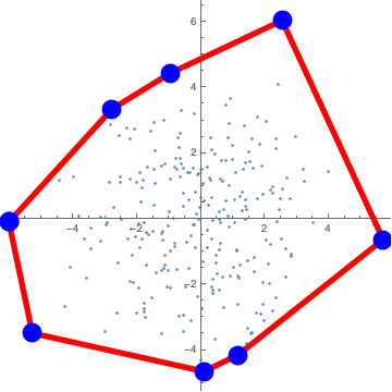
data=RandomReal[NormalDistribution[0,2],{250,2}];
Needs["ComputationalGeometry`"]

test=splitdata[data];
xx=Nest[Flatten[convexhull@@@#,1]&,test,3];
myline=Line/@Tally[xx[[All,1]]][[All,1]];
mypts=Point@Tally[xx[[All,1]]][[All,1,1]];

ListPlot[data,AspectRatio->1,
Epilog->{Red,Thickness[0.015],myline,Blue,PointSize[0.05],mypts}]
 

繼續閱讀全文　Mathematica 教學：Convex Hull

• 編輯文章
• 此文章網址
• 轉寄此文章
• 目前有0 意見

  

論文統計分析免煩惱，平均數比較、迴歸分析、信度、效度 CFA、結構方程是模型 SEM，一鍵搞定！ 

範例：本研究採量化研究，以XXX為研究對象，發放問卷XXX份，回收有效問卷XXX份，並以三山出版社所提供的 ThesisNoWorries 論文統計分析免煩惱 統計套件進行描述性統計、信效度分析、平均數比較、迴歸和相關分析、及結構方程式模型分析。

程式碼：https://github.com/chungyuandye/ThesisNoWorries

繼續閱讀全文　ThesisNoWorries Beta 0.3

• 編輯文章
• 此文章網址
• 轉寄此文章
• 目前有0 意見

Function acf(data As Range, k As Integer) As Double
Dim n As Integer
n = data.Rows.Count
Dim xbar As Double
xbar = Application.Average(data)
Dim sum1 As Double
sum1 = Application.SumProduct(data, data) - n * xbar * xbar
Dim sum2 As Double
sum2 = 0
For i = 1 To n - k
    sum2 = sum2 + (data.Cells(i) - xbar) * (data.Cells(i + k) - xbar)
Next
acf = sum2 / sum1
End Function

Function pacf(data As Range, k As Integer) As Double
Dim xx() As Double
ReDim xx(1 To k, 1 To k) As Double
For i = 1 To k
    For j = 1 To k
        xx(i, j) = acf(data, Abs(j - i))
    Next
Next
Dim yy() As Double
ReDim yy(1 To k, 1 To 1) As Double
For i = 1 To k
    For j = 1 To 1
        yy(i, 1) = acf(data, Abs(i))
    Next
Next 
pacf = Application.Index(Application.MMult(Application.MInverse(xx), yy), k, 1)
End Function

繼續閱讀全文　Excel：Calculate ACF and PACF in Excel

• 編輯文章
• 此文章網址
• 轉寄此文章
• 目前有0 意見

mytwoaxistikz[data__,{xmin_,xmax_,ymin_,ymax_},
mycolor__,{xlabel_,ylabel_},{rticks__,decimalr_,lticks__,decimall_},
linelabel__,linepos__,plotaspectratio_:1]:=Block[{temp=data,axis1,axis2,textpos,line},
axis1="
\\begin{axis}[
    yticklabel style={
        /pgf/number format/.cd,
            fixed,
            fixed zerofill,
            precision="<>ToString[decimall]<>",
    },
 scale only axis, 
 axis y line*=left, 
 xtick pos=left, 
 xscale="<>ToString[N@plotaspectratio]<>", 
 xmin="<>ToString[xmin]<>",xmax="<>ToString[xmax]<>",ymin="<>ToString[ymin]<>
 ",ymax="<>ToString[ymax]<>",
 xlabel="<>xlabel<>",ylabel="<>ylabel<>",
 ytick="<>ToString[lticks]<>"]\n";

textpos=StringJoin[Table["
 \\node[] at (axis cs:"<>ToString[linepos[[z,1]]]<>","<>ToString[linepos[[z,2]]]<>
 ") {"<>linelabel[[z]]<>"};",{z,Length@temp}]];

line=StringJoin[Table["
\\addplot[color="<>If[ListQ[mycolor[[z]]],
ToString[mycolor[[z,1]]]<>","<>ToString[mycolor[[z,2]]],
ToString[mycolor[[z]]]]<>",mark=none,line width=0.5mm] coordinates{\n"
 <>StringJoin["("<>ToString[#[[1]]]<>","<>ToString[#[[2]]]<>")\n"&/@temp[[z]]]<>
 "};\n\\addlegendentry{$G_{0}= "<>ToString[G0[[z]]]<>"$}",{z,Length@temp}]]
<>"\n\\end{axis}\n";

axis2="\n\\begin{axis}[ 
    yticklabel style={
        /pgf/number format/.cd,
            fixed,
            fixed zerofill,
            precision="<>ToString[decimalr]<>",
    },
 scale only axis, 
 axis y line*=right, 
 xtick pos=left, 
 xscale="<>ToString[N@plotaspectratio]<>", 
 xmin="<>ToString[xmin]<>",xmax="<>ToString[xmax]<>",ymin="<>ToString[ymin]<>
 ",ymax="<>ToString[ymax]<>",
 ytick="<>ToString[rticks]<>"]\n";

"\\begin{tikzpicture}"<>axis1<>textpos<>line<>axis2<>"\n\\end{axis}\n\\end{tikzpicture}"
]

繼續閱讀全文　Exporting graphics to TikZ format with Mathematica, Version 2

• 編輯文章
• 此文章網址
• 轉寄此文章
• 目前有0 意見

安裝 Ijupyter

python3 -m pip install --upgrade pip
python3 -m pip install jupyter

設定遠端連線 jupyter server，在python shell中執行

from notebook.auth import passwd; passwd()

生成修改設定檔

jupyter notebook --generate-config
vi ~/.jupyter/jupyter_notebook_config.py
c.NotebookApp.ip='*' #*表示所有IP，這裡設定ip為都可訪問  
c.NotebookApp.password = '填寫剛剛生成的密文'
c.NotebookApp.open_browser = False # 禁止notebook啟動時自動開啟瀏覽器
c.NotebookApp.port =9999 #指定訪問的埠，預設是8888。 

下載 configure-jupyter.wls

https://github.com/WolframResearch/WolframLanguageForJupyter

執行 wolframscript 安裝 WolframLanguageForJupyter

wolframscript configure-jupyter.wls add

啟動 Jupyter notebook

繼續閱讀全文　Mathematica 教學：使用 Jupyter Notebook 做為 Mathematica 操作環境

• 編輯文章
• 此文章網址
• 轉寄此文章
• 目前有0 意見

繼續閱讀全文　Excel 教學：符合條件整列變色

• 編輯文章
• 此文章網址
• 轉寄此文章
• 目前有0 意見

xx=Import["http://www.fishbase.org/summary/Decapterus-maruadsi.html","Table"];
StringJoin[#<>""&/@Cases[xx,{"Fisheries:",___},Infinity][[1,1;;-2]]]

繼續閱讀全文　Mathematica 教學：抓網頁特定資料

• 編輯文章
• 此文章網址
• 轉寄此文章
• 目前有0 意見

1. MI值調整
2. 項目分析報表修訂
3. 三構面中介模型報表修訂
4. 新增兩構面因果關係路徑模式

繼續閱讀全文　 ThesisNoWorryMed Beta 0.2

• 編輯文章
• 此文章網址
• 轉寄此文章
• 目前有0 意見

繼續閱讀全文　Temple trip

• 編輯文章
• 此文章網址
• 轉寄此文章
• 目前有0 意見

mytwoaxistikz[data__,{xmin_,xmax_,ymin_,ymax_},mycolor__,{xlabel_,ylabel_},{rticks__,lticks__},
linelabel__,linepos__,plotaspectratio_:1]:=Block[{temp=data,axis1,axis2,textpos,line},

axis1="
\\begin{axis}[
 scale only axis, 
 axis y line*=left, 
 xtick pos=left, 
 xscale="<>ToString[N@plotaspectratio]<>", 
 xmin="<>ToString[xmin]<>",xmax="<>ToString[xmax]<>",
 ymin="<>ToString[ymin]<>",ymax="<>ToString[ymax]<>",
 xlabel="<>xlabel<>",ylabel="<>ylabel<>",
 ytick="<>ToString[lticks]<>"]\n";

textpos=StringJoin[Table["
 \\node[] at (axis cs:"<>ToString[linepos[[z,1]]]<>","<>
ToString[linepos[[z,2]]]<>") {"<>linelabel[[z]]<>"};",
{z,Length@temp}]];

line=StringJoin[Table["
\\addplot[color="<>If[ListQ[mycolor[[z]]],
ToString[mycolor[[z,1]]]<>","<>ToString[mycolor[[z,2]]],
ToString[mycolor[[z]]]]<>",mark=none,line width=0.5mm] coordinates{\n"
 <>StringJoin["("<>ToString[#[[1]]]<>","<>ToString[#[[2]]]<>")\n"&/@temp[[z]]]<>"};",
{z,Length@temp}]]
<>"\n\\end{axis}\n";

axis2="\n\\begin{axis}[
 scale only axis, 
 axis y line*=right, 
 xtick pos=left, 
 xscale="<>ToString[N@plotaspectratio]<>", 
 xmin="<>ToString[xmin]<>",xmax="<>ToString[xmax]<>",
 ymin="<>ToString[ymin]<>",ymax="<>ToString[ymax]<>",
 ytick="<>ToString[rticks]<>"]\n";

"\\begin{tikzpicture}"<>axis1<>textpos<>line<>axis2<>"\n\\end{axis}\n\\end{tikzpicture}"
]

繼續閱讀全文　Exporting graphics to TikZ format with Mathematica

• 編輯文章
• 此文章網址
• 轉寄此文章
• 目前有0 意見

ThesisNoWorryMed Beta 0.1

目前提供三個變數的中介模型，一次跑完以下分析：

1. 三構面各分量表的項目分析
2. 三構面各分量表的Cronbach's alpha 信度及一階CFA的聚合效度 (AVE) 、收斂信度 (CR)及區別效度。
3. 三構面各分量表的人口統計差異性分析及事後比較。
4. 三構面的階層回歸中介效果檢定分析。
5. 三構面的結構方程式模型，SEM。

語法：

ThesisNoWorryMed[量表X, 量表M, 量表Y, X各分量表題數, Y各分量表題數, Z各分量表題數, X各分量表名稱, M各分量表名稱, Y各分量表名稱, 人口統計變數資料, 人口統計變數名稱]


ThesisNoWorryCFA[X, {5, 6, 4}, {X1, X2, X3}]

ThesisNoWorryMed[X, M, Y, {5, 6, 4}, {4, 5}, {3, 3}, {X1, X2, X3}, {M1, M2}, {Y1, Y2}, Dem, DemName]

繼續閱讀全文　ThesisNoWorryMed Beta 0.1

• 編輯文章
• 此文章網址
• 轉寄此文章
• 目前有0 意見

data=RandomVariate[BinormalDistribution[{1,2},{1.5,2},0.6],10000];

ListPlot[data,PlotRange->{{-5,8},{-5,8}},Axes->None,
Frame->True,AspectRatio->1,ImageSize->350,
FrameLabel->{
{Automatic,
Histogram[data[[All,2]],{-5,8,0.5},AspectRatio->0.2,
Axes->None,BarOrigin->Top,ImageSize->275]},
{Automatic,
Histogram[data[[All,1]],{-5,8,0.5},AspectRatio->0.2,
Axes->None,BarOrigin->Bottom,ImageSize->275]}}
]

Show[DensityHistogram[data,{0.5},ColorFunction->(White&),
Method->{"DistributionAxes"->"Histogram"}],ListPlot[data]]

繼續閱讀全文　Mathematica 教學：ListPlot with Histogram axes.

• 編輯文章
• 此文章網址
• 轉寄此文章
• 目前有0 意見

KKTMinimize[obj_,eqns_,ineqns_,variables_]:=
Block[{myrule,lambda,u,\[Lambda],Lagrange,eqnu,ineqnlam,
eqnus,ineqnlams,kkteqns,kktvars,kktans},
myrule={z_[i_]:>ToExpression[ToString[z]<>ToString[i]]};
eqnu=u[#]&/@Range[Length@eqns];
ineqnlam=\[Lambda][#]&/@Range[Length@ineqns];
eqnus=If[Length@eqns>=1,eqns.eqnu,0];
ineqnlams=If[Length@ineqns>=1,ineqns.ineqnlam,0];
kktvars=Flatten@{variables,eqnu,ineqnlam}/.myrule;
Lagrange=obj-eqnus-ineqnlams;
kkteqns=Flatten@{Thread[D[Lagrange,{variables}]==0],
Thread[eqns==0],Thread[ineqns<=0],
Thread[ineqns*ineqnlam==0],Thread[ineqnlam<=0]}/.
myrule;
If[MemberQ[PolynomialQ[#,kktvars]&/@kkteqns[[All,1]],False],
Print["KKT限制式均需為多項式。"],
kktans=Reduce[kkteqns,kktvars,
Backsubstitution->True]/.{And->List,Or->List,
Equal->Rule};
If[Length@Dimensions@kktans==1,{obj/.kktans,
kktans},{obj/.#,#}&/@kktans]]];

Plot[(1-Cos[x]/Cos[x/2])/x^2,{x,0.-10,Pi/2},
PlotRange->{{0,Pi/2},{0.3,0.5}},Frame->True,
FrameTicks->{{{0.3,0.5,{3/8,"3/8"},{4/Pi^2,"4/Pi^2"}},
None},{{0,Pi/2},None}},
GridLines->{None,{3/8,4/Pi^2}},GridLinesStyle->Dashed]

D[(1-Cos[x]/Cos[x/2])/x^2,x]//Simplify

D[(1-(Cos[x/2]^2-Sin[x/2]^2)/Cos[x/2])/x^2,x]//Simplify

D[4-4Sec[x/2]+3xTan[x/2]-4Tan[x/2]^2+xTan[x/2]^3,x]//TrigExpand//Simplify

(D[(6x-2Sin[x/2]-4Sin[x]-2Sin[(3x)/2]+Sin[2x]),x]//TrigExpand)
/.{Sin[z_]:>a,Cos[z_]:>b}

KKTMinimize[6+4a^2+2a^4-b+9a^2b-4b^2-12a^2b^2-3b^3+2b^4,{},
{-a,-b,a-1/Sqrt[2],1/Sqrt[2]-b,b-1},{a,b}]

Limit[(1-(Cos[x/2]^2-Sin[x/2]^2)/Cos[x/2])/x^2,x->0]

Limit[(1-(Cos[x/2]^2-Sin[x/2]^2)/Cos[x/2])/x^2,x->Pi/2]

Let f(x)=(1-cos(x)/cos(x/2))/x^2. Taking the first derivative of f(x) with respect to x yields d/dx f(x)=cos(x/2)*g(x)/(2x^3),
where g(x)=x*tan^3(x/2)-4*tan^2(x/2)+3*x*tan(x/2)-4*sec(x/2)+4. Because g'(x)=1/4*sec(x/2)^2*h(x) and h'(x)=k(x)=2*sin^4(x/2)+4*sin^2(x/2)+2*cos^4(x/2)-3*cos^3(x/2)-4*cos^2(x/2)-cos(x/2)-12*sin^2(x/2) *cos^2(x/2)+9*sin^2(x/2) cos(x/2)+6. Let a=sin(x/2) and b=cos(x/2). By Karush-Kuhn-Tucker conditions, we know that k(x) reaches its minimum at a=0 and b=1. This, together with the facts that h(0)=0, g(0)=0, and f(0)=0, indicates that f(x) is increasing in x, which also implies that 3/8<(1-Cos[x]/Cos[x/2])/x^2<4 br="" completes="" proof.="" the="" this="">

繼續閱讀全文　Mathematica 教學： Prove that 3/8< (1-cos(x)/cos(x/2))/x^2< 4/Pi^2 for all 0< x < Pi/2

• 編輯文章
• 此文章網址
• 轉寄此文章
• 目前有0 意見

Plot[1-3s^2+(1+s^2)Cosh[s],{s,0,Pi},Frame->True]
SeriesCoefficient[1-3s^2+(1+s^2)Cosh[s],{s,0,n}]
Normal[Series[1-3s^2+(1+s^2)Cosh[s],{s,0,5}]]
Minimize[2-(3s^2)/2+(13s^4)/24,s]
Solve[D[2-(3s^2)/2+(13s^4)/24,s]==0,s]

Since the coefficient in the n-th order of the taylor series of 1-3s^2+(1 + s^2)Cosh[s] is positive for every even term and is
zero for every odd term for all n>=3, it is obvious to see that 1-3s^2+(1+s^2)Cosh[s]>2-(3s^2)/2+(13s^4)/24>25/26, which implies that 1-3s^2+(1+s^2)Cosh[s]>0. This completes the proof.

繼續閱讀全文　Mathematica 教學： Prove that 1 - 3 s^2 + (1 + s^2) Cosh[s] >0.

• 編輯文章
• 此文章網址
• 轉寄此文章
• 目前有0 意見

mydate[date_]:=Block[{temp},
temp=Import[
"http://www.twse.com.tw/exchangeReport/MI_INDEX.html?date="<>ToString@date<>"&type=ALLBUT0999",
"JSON"];
{("data1"/.temp)[[All,{1,2,4,5}]],("data5"/.temp)[[All,
{1,2,3,4,5,6,7,8,9,11}]]}]

mydate[20170719][[1]] // TableForm
mydate[20170719][[2]] // TableForm

test=Quiet@{
{ToExpression@StringJoin@Characters[ToString@#][[1;;4]],
ToExpression@StringJoin@Characters[ToString@#][[5;;6]],
ToExpression@StringJoin@Characters[ToString@#][[7;;8]]},
mydate[#][[1,4]]}&/@Map[ToExpression@
StringJoin[ToString/@{#[[1]],
If[#[[2]]<10>ToString[#[[2]]],ToString[#[[2]]]],
If[#[[3]]<10>ToString[#[[3]]],
ToString[#[[3]]]]}]&,
DayRange["2017/05/1","2017/07/21"][[All,1]]]//Parallelize;

DateListPlot[{#[[1]],
ToExpression@StringReplace[#[[2,2]],","->""]}&/@
Select[test,Length@#[[2]]==4&],Filling->Bottom]


Block[{tempdata},
tempdata={#[[1]],ToExpression@StringReplace[#[[2,2]],","->""]}&/@
Select[test,Length@#[[2]]==4&];
DateListPlot[tempdata,Filling->Bottom,
Epilog->{Red,PointSize[0.025],Point[{tempdata[[#[[1]]]][[1]],#[[2]]}]&/@
FindPeaks[tempdata[[All,2]]]}]]
 

繼續閱讀全文　Mathematica 教學：抓取證交所股價資料

• 編輯文章
• 此文章網址
• 轉寄此文章
• 目前有0 意見

mylistplot[data_, xrange_, yrange_, pointsize_, colormap_, imagesize_] := 
  Module[{colors, styledData}, 
    colors = ColorData[colormap] /@ Rescale[data[[All, 2]], yrange];
    styledData = Style[#, colors[[#2]]] & @@@ Transpose[{data, Range[Length[data]]}];
    ListPlot[
      styledData, 
      PlotTheme -> "Detailed", 
      PlotStyle -> PointSize[pointsize], 
      PlotRange -> {xrange, yrange}, 
      Frame -> True, 
      ImageSize -> imagesize*GoldenRatio,
      PlotLegends -> Placed[
        BarLegend[{colormap, yrange}, LegendMarkerSize -> imagesize, 
        LegendMargins -> {{0, 0}, {0, 0}}],Right
      ]
    ]
  ]


mylistplot[iris, {2, 4}, {0, 2.5}, 0.015, "TemperatureMap", 225]

繼續閱讀全文　ListPlot with Colormap

• 編輯文章
• 此文章網址
• 轉寄此文章
• 目前有0 意見

Needs["RLink`"]

(* For Mac and MMA 10*)

SetEnvironment[ "DYLD_LIBRARY_PATH" ->"/Library/Frameworks/R.framework/Resources/lib"]
InstallR["RHomeLocation" -> "/Library/Frameworks/R.framework/Resources", "RVersion" -> 3];
REvaluate["R.version.string"]

(* Load packages*)

REvaluate["library(psych);"]
REvaluate["library(nortest);"]
REvaluate["library(GenABEL);"]

(* 因素分析，主成分法萃取，變異及大化法轉軸 *)

myfac=Map[REvaluate["{xx<-principal(iris[,1:4],nfactors="<>ToString[#]<>",
rotate=\"varimax\");xx$loadings}"]&,{2,3,4}];
myfac

(* 輸出因素負荷矩陣 *)

Reverse[SortBy[myfac[[1,1]],{#[[1]],#[[2]]}&]]//TableForm
TableForm/@myfac[[All,1]]


(* 因素分析資料*) 

fadata = {
{1, 1, 1, 1, 1, 1, 1, 1, 1, 1, 3, 3, 3, 3, 3, 4, 5, 6}, 
{1, 2, 1, 1, 1, 1, 2, 1, 2, 1, 3, 4, 3, 3, 3, 4, 6, 5}, 
{3, 3, 3, 3, 3, 1, 1, 1, 1, 1, 1, 1, 1, 1, 1, 5, 4, 6}, 
{3, 3, 4, 3, 3, 1, 1, 2, 1, 1, 1, 1, 2, 1, 1, 5, 6, 4}, 
{1, 1, 1, 1, 1, 3, 3, 3, 3, 3, 1, 1, 1, 1, 1, 6, 4, 5}, 
{1, 1, 1, 2, 1, 3, 3, 3, 4, 3, 1, 1, 1, 2, 1, 6, 5, 4}};

(* 定義資料*)

RSet["factor", Transpose@fadata];

(* 在R中計算相關係數矩陣，傳回MMA小數後四捨五入 *)

Round[REvaluate["cor(factor)"], 0.0001] // MatrixForm

(* 因素分析 *)

REvaluate["factanal(factor, factors = 3)$loadings"]

(* 輸出因素負荷矩陣 *)

TableForm[#[[1]], TableHeadings -> {None, #[[-1, -1, -1, -1]]}] & /@ 
{REvaluate["factanal(factor, factors = 3)$loadings"]} // Column
 
 
(* 迴歸分析 *)

REvaluate["{
data(iris)
reg <- lm( Sepal.Length ~ Species, data=iris )
summary.text <- capture.output(print( summary(reg)) )
}"]

StringJoin@Riffle[#, "\n"] &@REvaluate["{
data(iris)
reg <- lm( Sepal.Length ~ Species, data=iris )
summary.text <- capture.output(print( summary(reg)) )
}"]
 
(* 產生常態隨機變數 *)

mydata=REvaluate["rnorm(100,mean=0,sd=1)"]&/@Range[100]; 

(* MMA次數分配 *)

\[ScriptCapitalD] = HistogramDistribution[mydata[[1]]]  

(* MMA PDF & CDF *)

GraphicsRow[DiscretePlot[#[\[ScriptCapitalD], x], {x, -4, 4, .01}, 
PlotLabel -> #] & /@ {PDF, CDF}]

(* shapiro test, ks.test *)

shapiro[data_] := Block[{temp},
  RSet["temp", data];
  REvaluate[
 "{xx=shapiro.test(temp); yy=ks.test(temp,\"pnorm\",0,1); zz=lillie.test(temp); 
 c(xx$statistic,xx$p.value,yy$statistic,yy$p.value,zz$statistic,zz$p.value)}"][[1]] ]
 
RSet["rn1", RandomReal[{0, 10}, 1000]];
rn2 = RandomReal[NormalDistribution[0, 1], 1000];
REvaluate["rntransform(rn1)"] // Short
Histogram[#, Frame -> True] & /@ {rn2, REvaluate["rntransform(rn1)"]}
ShapiroWilkTest[#, {"TestStatistic", "PValue"}] & /@ {rn2, REvaluate["rntransform(rn1)"]} 


(* 利用RCurl擷取網路資料 *)

gosspost[n_]:=REvaluate["
{library(RCurl);
curl<-getCurlHandle();
curlSetOpt(cookie=\"over18=1\",followlocation=TRUE,curl=curl);
url<-\"https://www.ptt.cc/bbs/Gossiping/index" <> ToString[n] <> 
".html\";
html<-getURL(url,curl=curl)
}"][[1]];

Gossiping = 
  Cases[ImportString[
StringReplace[gosspost[#], {"\n" -> "", "\t" -> ""}], 
"XMLObject"],
  XMLElement[
 "div", {"class" -> "r-ent"}, {XMLElement[
"div", {"class" -> "nrec"}, {XMLElement[
  "span", {"class" -> "hl f2"}, {_}]}], 
  XMLElement["div", {"class" -> "mark"}, {}], 
  XMLElement[
"div", {"class" -> "title"}, {XMLElement[
  "a", {"shape" -> "rect", 
"href" -> postlink_}, {posttile_}]}], 
  XMLElement[
"div", {"class" -> "meta"}, {XMLElement[
  "div", {"class" -> "date"}, {_}], 
 XMLElement[
  "div", {"class" -> "author"}, {author_}]}]}] :> {postlink, 
 posttile, author},
  Infinity] & /@ Range[20861, 20862, 1];
  
Flatten[Gossiping, 1] // TableForm  

繼續閱讀全文　Use R within Mathematica

• 編輯文章
• 此文章網址
• 轉寄此文章
• 目前有0 意見

thesisnoworryhlm[構面1量表,構面2量表,構面3量表,{構面1各分量表題數},{構面2各分量表題數},{構面3各分量表題數},
{構面1各分量表變數名稱},{構面2各分量表變數名稱},{構面3各分量表變數名稱}]

thesisnoworryhlm[ddata[[All,1;;15]],ddata[[All,16;;24]],
ddata[[All,25;;30]],{5,6,4},{4,5},{3,3},
{X1,X2,X3},{M1,M2},{Y1,Y2}]

thesisnoworryanova[構面1量表,構面2量表,構面3量表,{構面1各分量表題數},{構面2各分量表題數},{構面3各分量表題數},
{構面1各分量表變數名稱},{構面2各分量表變數名稱},{構面3各分量表變數名稱},人口統計變量資料,{人口統計變量變數名稱}

thesisnoworryanova[ddata[[All,1;;15]],ddata[[All,16;;24]],
ddata[[All,25;;30]],{5,6,4},{4,5},{3,3},
{X1,X2,X3},{M1,M2},{Y1,Y2},
ddata[[All,{31,32,33}]],{"Sex","Age","Edu"}]

Thesis No Worry 程式資料檔

繼續閱讀全文　Thesis No Worry

• 編輯文章
• 此文章網址
• 轉寄此文章
• 目前有0 意見

1+2Sin[2x]+3Sin[3x]+4Sin[4x]/.{Plus->List,Sin[y_]->1}

繼續閱讀全文　How to get the coefficient of polynomial function

• 編輯文章
• 此文章網址
• 轉寄此文章
• 目前有0 意見

繼續閱讀全文　原生植物園

• 編輯文章
• 此文章網址
• 轉寄此文章
• 目前有0 意見